Research · ongoing · October 2026
Residual vision networks learn nearly autonomous flows
Integrating ConvNeXt, Swin and ResNet at any depth without fine-tuning, sharing one block across a whole stage, and the single channel that makes every trajectory look straighter than it is.
Jaume Ivars Grimalt · Mycrospace AI Research, Valencia · Trained on the Leonardo supercomputer (CINECA, EuroHPC)
In short
- Pretrained ConvNeXt-T, Swin-T, ResNet-50 and ResNet-101 can be run with 2 to 128 times more residual steps in their longest stage, with no fine-tuning, as long as the total integration time is kept. Accuracy converges to a continuous limit that is only 0.6 to 0.9 points below the original network.
- The networks are tuned to the error of a single Euler step: any more accurate solver at the training step size lands directly on that limit.
- Interpolating weights linearly between consecutive blocks fails in every model, losing 6.6 to 23.3 points. Only piecewise-constant weights work.
- A ConvNeXt-T whose nine stage-3 blocks are a single shared block reaches 80.34% on ImageNet against 80.96%, with roughly a third fewer parameters. Its accuracy depends almost only on the integration time, not on the number of steps.
- Adding a zero-initialised delta per block on top of the shared block, and fine-tuning, gives 81.25%: above both the shared and the original network.
- The straight, almost one-dimensional trajectories of ConvNeXt are an artefact of one massive channel that holds 98 to 99% of the state's energy. Without it the dynamics are rotational and multi-dimensional.
1. The idea
A residual block computes [1]. Read with a step size of one, that is exactly one step of the explicit Euler method for the ODE [2, 3, 4]. Neural ODEs took the idea to its conclusion and replaced the stack of blocks with a solver [5]. Whether ordinary, discretely trained networks really behave like that discretisation is a separate question, and the answer depends on how they were trained [6].
The reading I use is that a residual stage is a sum of blocks, and each block is an integral of its own vector field. Write the residual of block as
Then the native network is one Euler step of size 1 per block. The continuous object behind it is the sum of those integrals:
The sum is the stack of residual blocks. The integral is the interpolation of that block: instead of taking one Euler step of size 1, integrate over the unit interval with a finer solver, keeping the horizon of each block equal to 1. Equivalently, block by block,
I test this on the long stage of pretrained networks, without retraining: stage 3 has blocks in ConvNeXt-T [7], 6 in Swin-T [8], 5 in ResNet-50 and 22 in ResNet-101. If the network is an Euler discretisation of a smooth flow, refining the integral should converge. If each block is an arbitrary map that only works with its exact input, it should collapse. I also integrate with RK2 and RK4 [9] to locate the continuous limit of (2).
How the integral is discretised is the interpolation. Plain interpolation keeps the field piecewise constant on each block: Euler steps of size ,
Bilinear interpolation replaces by a blend of consecutive blocks, which is what most continuous-depth work assumes [10, 11]. In weight space that is
All accuracies are top-1 on the 50,000 ImageNet-1k validation images [12]. ConvNeXt-T (with and without drop path) is my own run, trained from scratch for 300 epochs with timm augmentation [13]. Swin-T and the ResNets use the torchvision weights [14].
2. Refining pretrained networks
All five networks behave like Euler discretisations. Accuracy decreases monotonically as the step shrinks and flattens out at a well-defined limit, the same one RK4 reaches. The limit is always slightly below the original network.
- ConvNeXt-T
- ConvNeXt-T, no drop path
- Swin-T
- ResNet-50
- ResNet-101
| Model | Original | RK4 at step 1 | Euler R = 128 | ODE limit | Gap |
|---|---|---|---|---|---|
| ConvNeXt-T | 80.96 | 80.23 | 80.24 | 80.23 | −0.73 |
| ConvNeXt-T, no drop path | 79.27 | 76.98 | 77.02 | 76.96 | −2.31 |
| Swin-T | 81.08 | 80.33 | 80.34 | 80.32 | −0.76 |
| ResNet-50 | 80.34 | 79.42 | 79.45 | 79.43 | −0.91 |
| ResNet-101 | 81.67 | 81.06 | 81.06 | 81.05 | −0.62 |
ODE limit: RK4 with R = 128. Gap: ODE limit minus original.
Two things stand out. First, the horizon is what matters. Repeating each block ten times without shrinking the step, which integrates ten times longer, destroys every network: 0.1% for ConvNeXt, 1% for Swin. Second, the networks are tuned to Euler's error. Swapping in RK2 or RK4 at the training step size gives the continuous limit straight away and loses between 0.15 and 2.5 points. A single Euler step of size one is not a poor approximation of the ODE. It is the function that was trained, and the ODE is a slightly worse approximation of it.
3. Plain versus bilinear interpolation
Interpolating weights between consecutive blocks fails in every model, and the more steps you take, the worse it gets.
- ConvNeXt-T
- ConvNeXt-T, no drop path
- Swin-T
- ResNet-50
- ResNet-101
At R = 128, bilinear loses 6.58, 19.58, 8.20, 11.68, 23.33 points against plain, in the order of the table above. The cause is permutation symmetry. Two consecutive blocks are not aligned neuron by neuron, so the midpoint of their weights is not a functional block that lies between them [15, 16]. The damage also ranks the models by how similar consecutive blocks are: ConvNeXt with drop path and Swin are the smoothest, while ResNet-101 and ConvNeXt without drop path are the roughest.
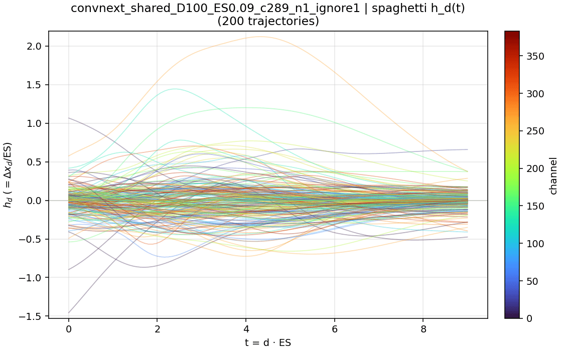
You can see it in the residual field. Each curve below is one channel of h = Δx/Δt, averaged over space, along the nine blocks of ConvNeXt-T at R = 100, for a single validation image (a snow leopard).
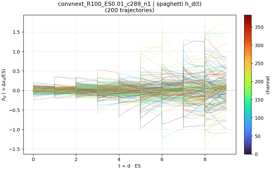
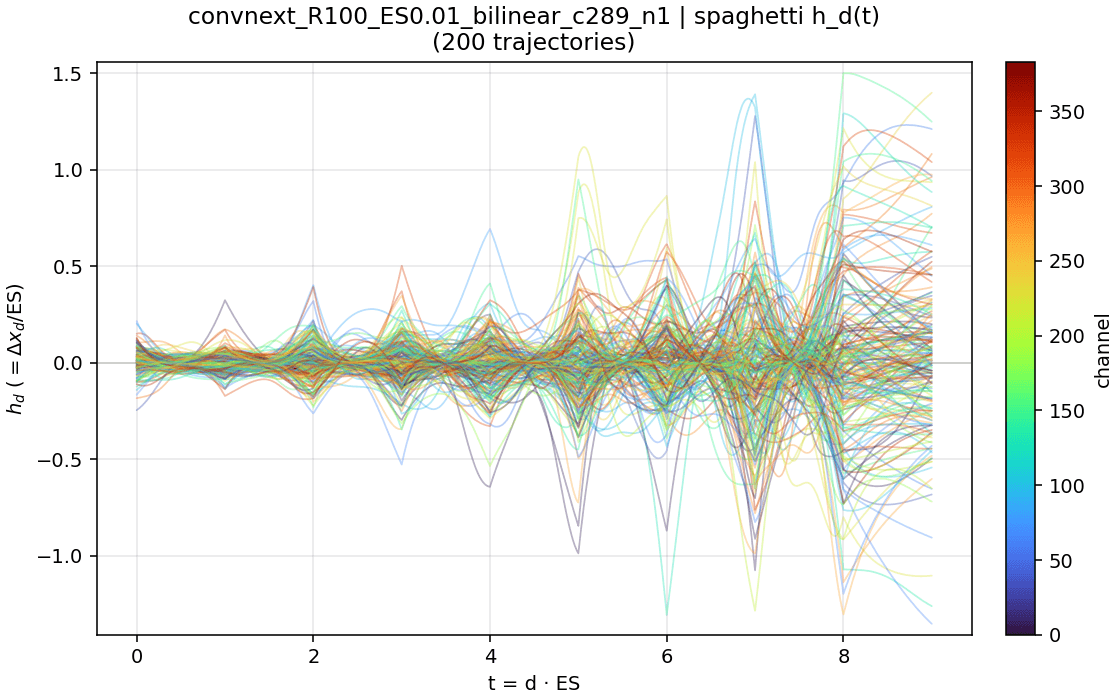
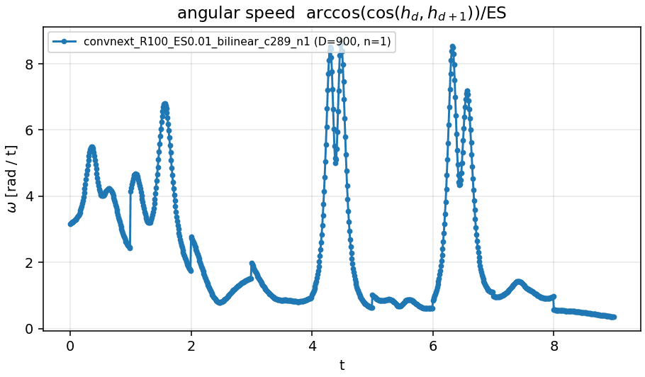
In numbers, measured over 500 images: bilinear keeps the global shape of the trajectory (its straightness and dimensionality barely change) but multiplies local curvature by 6 to 12 and angular speed by 4 to 7, and doubles the distance to the native trajectory.
4. One block for the whole stage
If stage 3 really integrates a smooth flow, one block should be able to define the vector field for the whole stage. So I trained a ConvNeXt-T in which the nine stage-3 blocks are the same block applied nine times, with the same recipe as the baseline: 300 epochs on ImageNet-1k. Weight sharing across depth is not new [17, 18], but here it is a direct test of the ODE reading.
- ConvNeXt-T
- ConvNeXt-T, no drop path
- Shared stage 3 (1 block × 9)
The shared network reaches 80.34% against 80.96%, a cost of 0.62 points. Stage 3 goes from nine blocks to one, which removes about 9.6M of ConvNeXt-T's 28.6M parameters.
Accuracy depends on the integration time, not on the number of steps
With a single field, depth D and step Δt can be chosen freely at inference, and the integration time is T = D · Δt. The network was trained with D = 9 and Δt = 1, so T = 9. Keeping T = 9 and changing D:
- Euler (RK1)
- RK2
- RK4
The gap from Euler to the continuous limit is −0.22 points, three times smaller than in the unshared ConvNeXt (−0.73): sharing weights produces a more genuine ODE. With large steps the order of the solver matters a lot. At D = 4, RK4 gets 78.9% and Euler 67.8%, and Euler with two steps of 4.5 is unstable (5.9%). RK4 reaches the limit from D ≈ 5, RK2 from about 18 and Euler only from about 256.
- Fixed step 1, more steps (T = D)
- 9 steps, varying step size (T = 9 · step)
Integrating too short or too long degrades smoothly near T = 9 and collapses far from it: 49% at T = 32 with unit steps, and 0.3% at T = 128. The classification head expects the state reached after exactly that much time.
5. Shared block plus per-block deltas
Sharing costs 0.6 points. The question that gives the project its name is whether that gap can be closed without giving up the shared structure. Each block k gets its own offset on top of the shared weights:
The deltas cover every parameter of the block: depthwise convolution, LayerNorm, both pointwise layers and the layer scale. They start at zero from the shared checkpoint, so epoch 0 is exactly the shared network, and they have their own weight decay pulling them back towards it. Then the whole model is fine-tuned.
- Δ, 9 steps, peak LR 1e-3, 50 epochs
- Δ, 9 steps, peak LR 1e-4, 100 epochs
- Δ, unrolled to 27 steps of 1/3, LR 1e-5 (running)
With a peak learning rate of 10⁻³ for 50 epochs, the delta model reaches 81.25%, +0.91 over the shared network and +0.29 over the original. A gentler schedule (10⁻⁴, 100 epochs) stays at 80.57%. The deltas do not stay small. By the end of the best run they average 27% of the norm of the shared weights.
- mean ‖δₖ‖ / ‖θ_shared‖ over blocks and layers
Two caveats, to be fair to the baseline. The delta model has as many stage-3 parameters as the original plus one block, so it is a reparametrisation, not a compression. And it has seen 50 more epochs than the original. What it shows is that a shared field plus per-block corrections is a better starting point than nine independent blocks. Whether the deltas can be made sparse or low-rank, recovering the parameter savings, is the next step.
6. What the trajectories look like
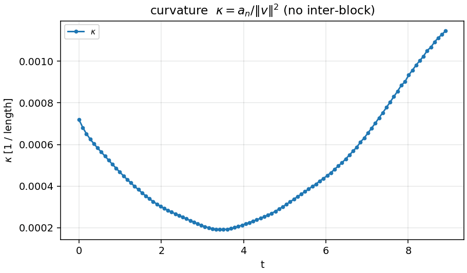
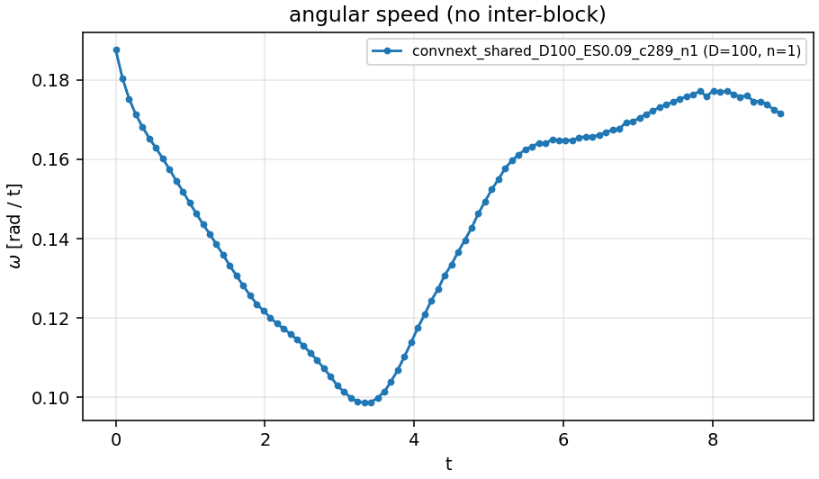
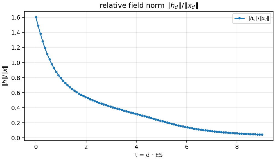
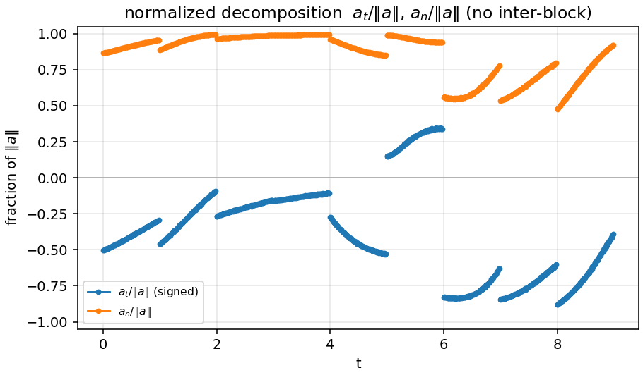
To compare networks beyond accuracy I measure the geometry of the path the state takes through stage 3: norms of and , angular speed of , tangential and normal acceleration, curvature, straightness (net displacement over path length; 1 for a straight line), and the participation ratio of the trajectory, its effective number of dimensions. Everything was first computed on one image (ImageNet val #644, a snow leopard), then repeated on a suite of 500 validation images, one from each of 500 random classes (seed 0; the same 500 images in every run).
The single image was representative. Every metric of that image falls within about 1.5 standard deviations of the 500-image mean, and the spread between images is small (). The geometry belongs to the network, not to the input. The numbers in the tables below are that N=500 mean.

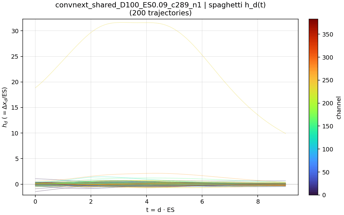
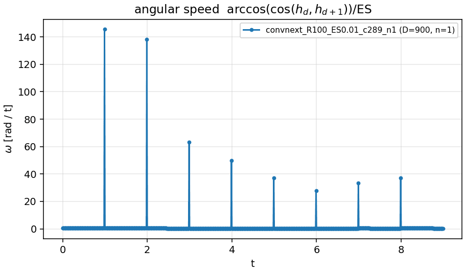
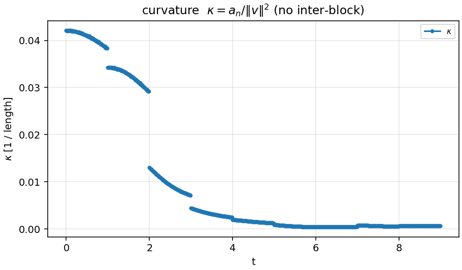
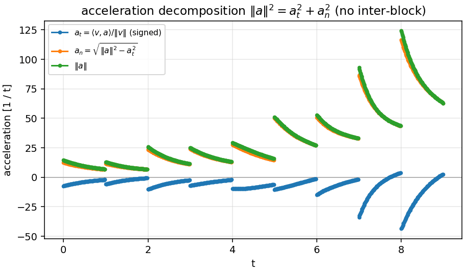
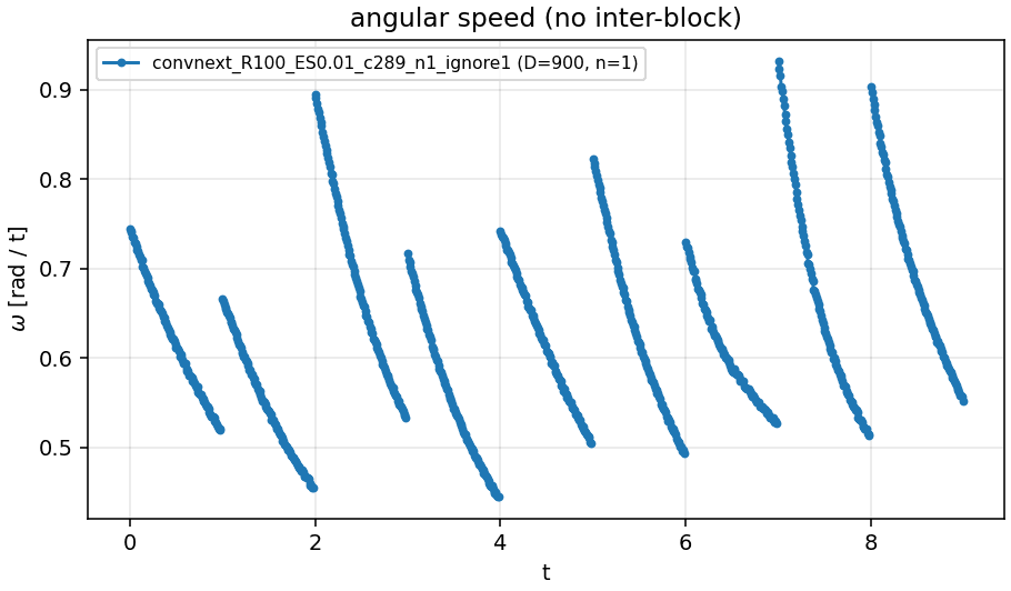
With all channels included, every ConvNeXt looks like an almost perfectly straight, one-dimensional flow, and there is a clear ranking: shared, then ConvNeXt, then Swin, then the ResNets. ResNet-101 follows a very tortuous path in about 20 effective dimensions. The unshared ConvNeXt shows a sawtooth pattern: inside each block h contracts, and at each block boundary it jumps by 10² to 10⁴ times the within-block acceleration.
Dynamics and geometry
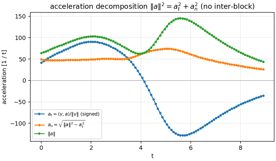
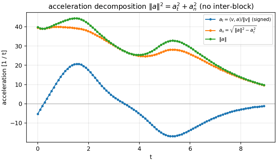
Write for the residual velocity and for its acceleration. The tangential and normal parts are
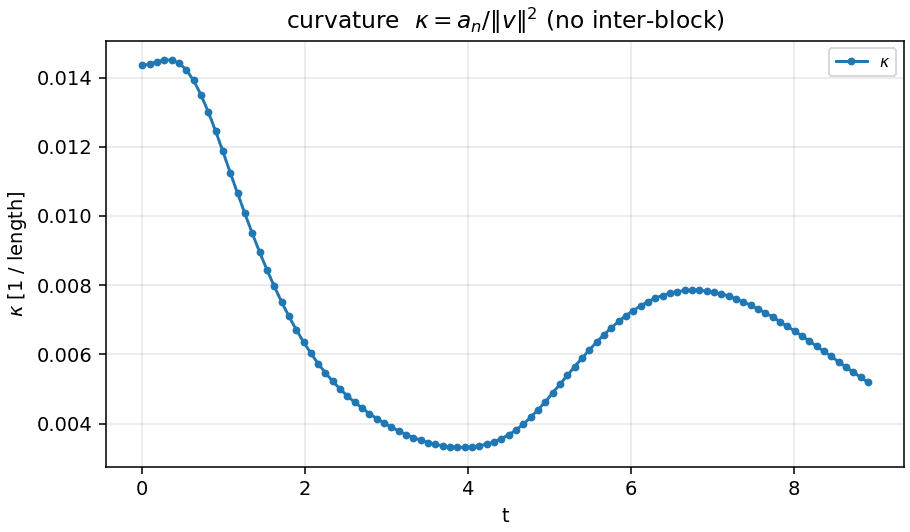
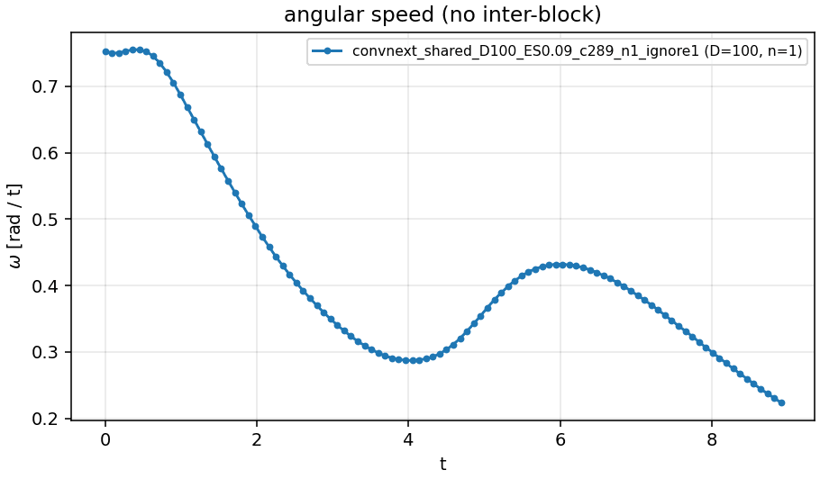
is signed: negative means the trajectory is braking ( shrinks). is a norm, so always positive, and . Angular speed is . The panels below drop the single step between blocks, so they show the intra-block flow; the panel that keeps those steps is labelled as such.
7. Massive activations and the ignore path
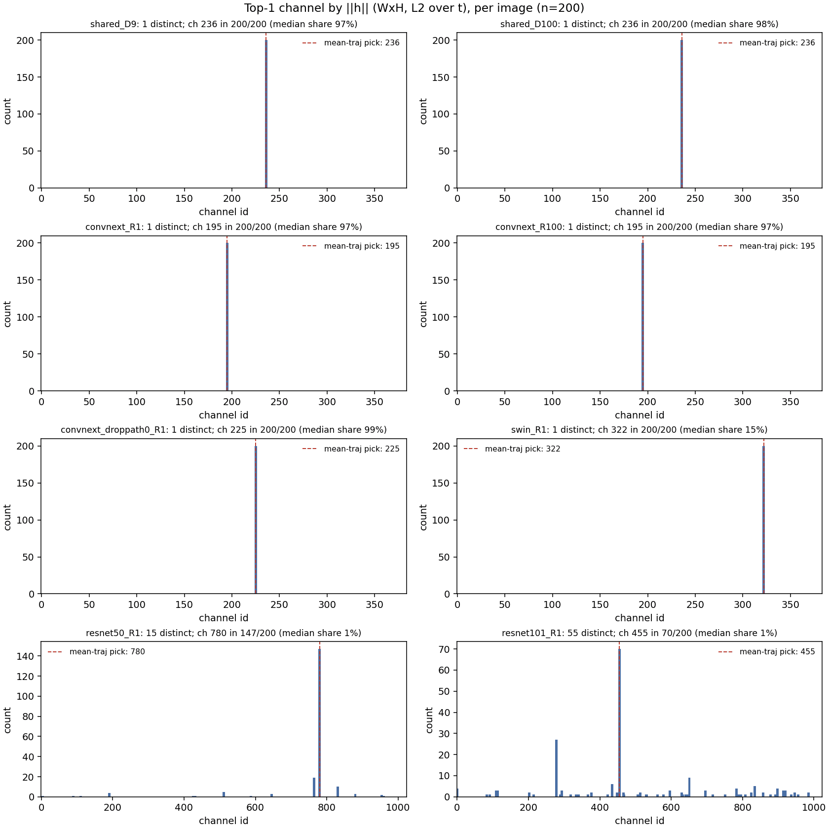
The straight lines are mostly one channel: a massive activation [19]. At the exit of stage 3 in the shared network, channel 236 has a norm of 3,570; the next largest has 140. It is the same channel in all 200 images I checked, and it holds a median 98% of the energy of the state.
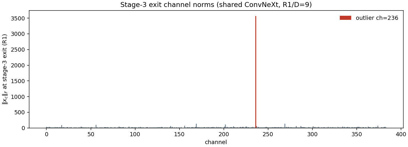
The same phenomenon appears in all three ConvNeXts (channels 236, 195 and 225, with 97 to 99% of the energy). Swin has a moderate one, at about 15%, and the ResNets have none: their top channel changes from image to image and carries about 1%. They are close relatives of the high-norm tokens in vision transformers [20]. One difference: in the shared network the channel dominates from the first step, while in the unshared ConvNeXt it emerges with depth, from 5% of at the start to 96% at the end.
The ignore path: drop the channel from the metric, not from the ODE
The ignore path (_ignore1 in the experiment suite) leaves the network untouched and only removes the massive channel when the trajectory metrics are computed. That is not the same as zeroing the channel inside the residual step, which I come back to below. On N=500, ignoring it changes ConvNeXt completely and Swin almost not at all.
| Model | Ignore | R | σ(R) | PR depth | PR spatial | κ | ω | aₙ/‖a‖ | aₜ/‖a‖ | cos(x₀,x_T) | cos(h₀,h_T) |
|---|---|---|---|---|---|---|---|---|---|---|---|
| Shared stage 3 | — | 0.970 | 0.008 | 1.09 | 1.03 | 0.0005 | 0.15 | 0.58 | -0.07 | 0.67 | 0.73 |
| Shared stage 3 | ch 236 | 0.776 | 0.020 | 1.94 | 6.24 | 0.0075 | 0.41 | 0.95 | -0.06 | 0.31 | -0.06 |
| ConvNeXt-T | — | 0.938 | 0.010 | 1.19 | 1.13 | 0.0098 | 0.34 | 0.87 | -0.38 | 0.48 | 0.17 |
| ConvNeXt-T | ch 195 | 0.502 | 0.011 | 3.46 | 32.00 | 0.0210 | 0.61 | 0.97 | -0.21 | 0.21 | 0.02 |
| ConvNeXt-T, no drop path | — | 0.934 | 0.010 | 1.04 | 8.76 | 0.0200 | 0.56 | 0.96 | 0.04 | 0.33 | 0.27 |
| ConvNeXt-T, no drop path | ch 225 | 0.438 | 0.012 | 3.20 | 29.50 | 0.0280 | 0.84 | 0.98 | 0.10 | 0.17 | 0.01 |
| Swin-T | — | 0.825 | 0.014 | 1.17 | 6.15 | 0.0042 | 0.50 | 0.89 | -0.39 | 0.09 | 0.04 |
| Swin-T | ch 322 | 0.812 | 0.016 | 1.17 | 7.31 | 0.0044 | 0.51 | 0.89 | -0.39 | 0.08 | 0.03 |
| ResNet-50 | — | 0.396 | 0.012 | 4.94 | 5.84 | 0.0024 | 0.63 | 0.90 | -0.41 | 0.60 | -0.08 |
| ResNet-101 | — | 0.169 | 0.005 | 19.66 | 12.10 | 0.0022 | 0.54 | 0.93 | -0.31 | 0.48 | -0.04 |
N=500, one ImageNet validation image per class, same 500 images in every run. Fine Euler (R=100 or D=100). R is straightness (N/L). κ and ω are intra-block means. ResNets have no massive channel, so there is no ignore path for them.
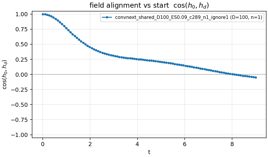
With every channel, the ranking in straightness is shared 0.97 > ConvNeXt 0.94 ≈ no-drop-path 0.93 > Swin 0.83 > ResNet-50 0.40 > ResNet-101 0.17. After the ignore path it becomes Swin 0.81 > shared 0.78 > ConvNeXt 0.50 > no-drop-path 0.44 > ResNet-50 0.40 > ResNet-101 0.17. The unshared ConvNeXt without its channel is almost as tortuous as ResNet-50; Swin is the unshared network whose straightness is real. In the shared network more than 90% of the acceleration becomes normal: rotates until it ends up orthogonal to where it started (), while fades from 0.42 to 0.09. A drift that turns and dies out.
Zeroing versus ignoring
Zeroing writes the channel to 0 after every residual step of the shared network, so the ODE itself changes. That drops accuracy from 80.34% to 67.81%. Zeroing a random channel instead costs nothing (mean 80.25% over 20 channels). The same holds at ten times the resolution (from 80.14% to 67.59%).
The ignore path and this zeroing agree on the other 383 channels to within 0.5% on every metric (straightness 0.7944 vs 0.7947, path length, participation ratios, mean curvature). The channel does not feed back into the rest of the stage-3 field, so it is not an internal clock that reads. Its effect is downstream: holding 98% of the energy, it sets the variance that the LayerNorm before downsampling divides by. Remove it and the scale of everything else changes about 7×, a distribution shift for stage 4. Whether it carries information about the image, or acts as a near-constant bias and scale, is still open.
8. Is drop path the reason?
Stochastic depth [21] randomly skips blocks during training, so every block has to be optional. That should push towards small updates that agree with their neighbours, which is what an ODE needs. Residual networks are already known to tolerate dropped and reordered layers [22, 23, 24]. ConvNeXt-T trained without drop path tests the idea directly:
| With drop path 0.1 | Without | Difference | |
|---|---|---|---|
| Original accuracy | 80.96 | 79.27 | −1.69 |
| ODE limit (RK4) | 80.23 | 76.96 | −3.27 |
| Gap to the limit | −0.73 | −2.31 | 3.2× larger |
| Bilinear, R = 128 | 73.66 | 57.44 | −16.2 |
Without drop path, the gap to the continuous limit triples, bilinear interpolation collapses, and the blocks stop contracting. It is the only network whose trajectory accelerates inside each block and whose ‖h‖/‖x‖ grows with depth, from 0.39 to 0.65. But drop path is not a necessary condition, since Swin and both ResNets converge with similar gaps. The Euler-like behaviour seems to be generic to deep residual networks, and drop path strengthens it.
9. Open questions
- Finish the 27-step delta run, and the shared networks with 27 steps and with every stage shared, and run the depth, step and solver ablations on them.
- Make the deltas sparse or low-rank, so the delta model recovers the parameter savings of sharing.
- Pin down the massive channel. Replace it by its dataset mean instead of zero, which separates bias from information. Replace it by its value at a different time, which tests a clock read by stage 4. Zero it only at the exit of stage 3. Fit a linear probe of the class on it.
- Repeat the zeroing on the unshared ConvNeXt and on Swin, where the channel emerges with depth.
- Close the causal question about drop path with intermediate rates and a shared network trained without it.
- Interpolate in function space, (1 − α) fk(x) + α fk+1(x), which needs no weight alignment, or in weight space after aligning consecutive blocks [16].
The training framework and the from-scratch ConvNeXt run this builds on are written up in ConvNeXt-V1 from scratch on Leonardo. If you work on continuous-depth models or massive activations and want to compare notes, write to jaume@jaumeivars.com.
References
- [1]K. He, X. Zhang, S. Ren, J. Sun. Deep Residual Learning for Image Recognition. CVPR, 2016.
- [2]W. E. A Proposal on Machine Learning via Dynamical Systems. Communications in Mathematics and Statistics 5(1), 2017.
- [3]E. Haber, L. Ruthotto. Stable Architectures for Deep Neural Networks. Inverse Problems 34(1), 2017.
- [4]Y. Lu, A. Zhong, Q. Li, B. Dong. Beyond Finite Layer Neural Networks: Bridging Deep Architectures and Numerical Differential Equations. ICML, 2018.
- [5]R. T. Q. Chen, Y. Rubanova, J. Bettencourt, D. Duvenaud. Neural Ordinary Differential Equations. NeurIPS, 2018.
- [6]M. E. Sander, P. Ablin, G. Peyré. Do Residual Neural Networks discretize Neural Ordinary Differential Equations? NeurIPS, 2022.
- [7]Z. Liu, H. Mao, C.-Y. Wu, C. Feichtenhofer, T. Darrell, S. Xie. A ConvNet for the 2020s. CVPR, 2022.
- [8]Z. Liu, Y. Lin, Y. Cao, H. Hu, Y. Wei, Z. Zhang, S. Lin, B. Guo. Swin Transformer: Hierarchical Vision Transformer using Shifted Windows. ICCV, 2021.
- [9]E. Hairer, S. P. Nørsett, G. Wanner. Solving Ordinary Differential Equations I: Nonstiff Problems (2nd ed.). Springer, 1993.
- [10]B. Chang, L. Meng, E. Haber, F. Tung, D. Begert. Multi-level Residual Networks from Dynamical Systems View. ICLR, 2018.
- [11]A. F. Queiruga, N. B. Erichson, D. Taylor, M. W. Mahoney. Continuous-in-Depth Neural Networks. arXiv preprint, 2020.
- [12]J. Deng, W. Dong, R. Socher, L.-J. Li, K. Li, L. Fei-Fei. ImageNet: A Large-Scale Hierarchical Image Database. CVPR, 2009.
- [13]R. Wightman. PyTorch Image Models. GitHub repository, 2019.
- [14]TorchVision maintainers and contributors. TorchVision: PyTorch's Computer Vision library. GitHub repository, 2016.
- [15]R. Entezari, H. Sedghi, O. Saukh, B. Neyshabur. The Role of Permutation Invariance in Linear Mode Connectivity of Neural Networks. ICLR, 2022.
- [16]S. K. Ainsworth, J. Hayase, S. Srinivasa. Git Re-Basin: Merging Models modulo Permutation Symmetries. ICLR, 2023.
- [17]M. Dehghani, S. Gouws, O. Vinyals, J. Uszkoreit, Ł. Kaiser. Universal Transformers. ICLR, 2019.
- [18]Z. Lan, M. Chen, S. Goodman, K. Gimpel, P. Sharma, R. Soricut. ALBERT: A Lite BERT for Self-supervised Learning of Language Representations. ICLR, 2020.
- [19]M. Sun, X. Chen, J. Z. Kolter, Z. Liu. Massive Activations in Large Language Models. COLM, 2024.
- [20]T. Darcet, M. Oquab, J. Mairal, P. Bojanowski. Vision Transformers Need Registers. ICLR, 2024.
- [21]G. Huang, Y. Sun, Z. Liu, D. Sedra, K. Q. Weinberger. Deep Networks with Stochastic Depth. ECCV, 2016.
- [22]A. Veit, M. Wilber, S. Belongie. Residual Networks Behave Like Ensembles of Relatively Shallow Networks. NeurIPS, 2016.
- [23]K. Greff, R. K. Srivastava, J. Schmidhuber. Highway and Residual Networks learn Unrolled Iterative Estimation. ICLR, 2017.
- [24]S. Jastrzębski, D. Arpit, N. Ballas, V. Verma, T. Che, Y. Bengio. Residual Connections Encourage Iterative Inference. ICLR, 2018.