Research · ongoing · October 2026
All skip-connections can be expanded indefinitely
An analysis of representation dynamics in vision models with differential geometry
Jaume Ivars Grimalt · Mycrospace AI Research, Valencia · Trained on the Leonardo supercomputer (CINECA, EuroHPC)
Take a photo of a snow leopard, push it through a ConvNeXt and stop at the entrance of its third stage. At that point the network no longer holds an image. It holds 384 channels on a 14 × 14 grid: 75,264 numbers. I find it useful to stop thinking of them as a feature map and to think of them as a single point . The nine blocks of the stage move that point, and where it ends up is, in large part, what the network decides the image is.
Every block moves it in the same way. It looks at where the point is, computes a direction, and adds it:
Anyone who has written a numerical solver recognises that line. It is one step of Euler's method, with step size 1, for the differential equation . Read like that, is not a layer but a vector field: a rule that pins an arrow, a velocity, on every location of that 75,264-dimensional space. The point does not jump from layer to layer; it is carried along by the arrows, and the network is the path it draws. The idea is older than this project [2, 3, 4, 5]. What I wanted to know is whether it is literally true of the networks we actually train, and what it buys us if it is.
The test is almost embarrassingly simple. If block really is one Euler step of a field , I should be able to replace it by a hundred steps of size 1/100 and land in nearly the same place. I can, in ConvNeXt, Swin and ResNet, without retraining a single weight, and as far as I push it. That is the title: every skip connection can be expanded indefinitely. The interesting part is what the expansion gives in return. Nine snapshots become a continuous curve , and the question stops being “what does each block output?” and becomes “how does the point move?” How fast, whether it accelerates or brakes, whether it goes straight or turns. Those are questions for differential geometry: velocity , acceleration , split into a tangential part that changes the speed and a normal part that changes the direction, and curvature . None of them can be estimated from nine samples. All of them can from nine hundred.
Seen this way, two kinds of network turn out to move in two very different ways. When the nine blocks of the stage are one and the same block, which I call weight-tied or shared, there is a single field and it does not depend on time:
That is an autonomous system. The arrows are fixed in space, and the point simply follows them. Its velocity is continuous by construction, and what it does, for every image I have looked at, is launch, push and brake: the speed rises, peaks around and fades, while the classes fan out from a common origin (Figure 1, left).
In the original network every block has its own weights, so the field is
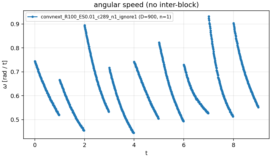
autonomous within each unit of time and replaced by a different one at every integer : piecewise autonomous. Inside a block the point glides along a smooth curve. At the boundary, all the arrows under it change at once, and so does its velocity. The jumps are large. Across a block boundary 45% of the coordinates reverse the sign of their velocity, the displacements of consecutive blocks are almost orthogonal (cosine 0.17 over 500 images), and the speed climbs in steps from about 17 to over 100 (Figure 1, right). Both networks classify equally well. One gets there by flowing, the other by a sequence of pushes in unrelated directions that partly undo each other.
A warning that applies to every picture on this page: one channel of ConvNeXt holds 98 to 99% of the energy of the state, and left in, it makes every trajectory look like a straight line. I leave it out of the measurements, not out of the network; section 7 explains why. The rest of the page builds the argument step by step. It shows that refining depth works and how far, why the weights inside a block must stay constant, that one shared block is enough for a whole stage, and then what the trajectories look like at high resolution.
In short
- Pretrained ConvNeXt-T, Swin-T, ResNet-50 and ResNet-101 can be run with 2 to 128 times more residual steps in their longest stage, with no fine-tuning, as long as the total integration time is kept. Accuracy converges to a continuous limit that is only 0.6 to 0.9 points below the original network.
- The networks are tuned to the error of a single Euler step: any more accurate solver at the training step size lands directly on that limit.
- Interpolating weights linearly between consecutive blocks fails in every model, losing 6.6 to 23.3 points. Only piecewise-constant weights work.
- A ConvNeXt-T whose nine stage-3 blocks are a single shared block reaches 80.34% on ImageNet against 80.96%, with roughly a third fewer parameters. Its accuracy depends almost only on the integration time, not on the number of steps.
- Expanding the skip connections is a microscope. The refined network keeps the original function, but samples its trajectory 100 times more densely, which is what velocities, accelerations and curvatures need. At that resolution the shared network is a smooth flow that accelerates and brakes, and the original network is a sequence of nearly orthogonal pushes.
- Over 500 images, consecutive blocks of the original ConvNeXt-T move the state in almost unrelated directions (cosine 0.17), and 45% of the coordinates reverse direction from one block to the next. Half of all the motion in stage 3 cancels out. The shared block wastes 19%.
- The straight, almost one-dimensional trajectories of ConvNeXt are an artefact of one massive channel that holds 98 to 99% of the state's energy. Without it the dynamics are rotational and multi-dimensional.
- Adding a zero-initialised delta per block on top of the shared block, and fine-tuning, gives 81.25%: above both the shared and the original network.
1. The idea
Now more carefully. A residual block computes [1]. Read with a step size of one, that is exactly one step of the explicit Euler method for the ODE [2, 3, 4]. Neural ODEs took the idea to its conclusion and replaced the stack of blocks with a solver [5]. Whether ordinary, discretely trained networks really behave like that discretisation is a separate question, and the answer depends on how they were trained [6].
The reading I use is that a residual stage is a sum of blocks, and each block is an integral of its own vector field. Write the residual of block as
Then the native network is one Euler step of size 1 per block. The continuous object behind it is the sum of those integrals:
The sum is the stack of residual blocks. The integral is the interpolation of that block: instead of taking one Euler step of size 1, integrate over the unit interval with a finer solver, keeping the horizon of each block equal to 1. Equivalently, block by block,
I test this on the long stage of pretrained networks, without retraining: stage 3 has blocks in ConvNeXt-T [7], 6 in Swin-T [8], 5 in ResNet-50 and 22 in ResNet-101. If the network is an Euler discretisation of a smooth flow, refining the integral should converge. If each block is an arbitrary map that only works with its exact input, it should collapse. I also integrate with RK2 and RK4 [9] to locate the continuous limit of (2).
How the integral is discretised is the interpolation. Plain interpolation keeps the field piecewise constant on each block: Euler steps of size ,
Bilinear interpolation replaces by a blend of consecutive blocks, which is what most continuous-depth work assumes [10, 11]. In weight space that is
What I propose
The title is the claim: every skip connection can be expanded indefinitely. Take any block of a trained network and replace it by applications of . Nothing is retrained, no weight is changed, and the result is still a working classifier for any , all the way to the continuous limit. That one operation supports four things:
- Evidence that residual blocks are one-step ODE solvers. If they were arbitrary maps that only work with their exact input, splitting them would break the network. It does not, in ConvNeXt, Swin or ResNet (section 2), but only if the weights inside each block are kept constant (section 3).
- A smaller network with the same dynamics. If the stage integrates a flow, one block should be enough to define it. A ConvNeXt-T with a single shared stage-3 block, trained from scratch, is within 0.6 points of the original (section 4).
- A microscope for representation dynamics. The expanded network samples the path of the representation 100 times more densely, so velocity, acceleration, curvature and the timing of every coordinate become measurable (sections 5 and 6). This is the part I find most useful, and the reason the paper analyses trajectories with differential geometry.
- A better way to build the discrete network. What the microscope shows, that independent blocks spend half their motion undoing each other, motivates a shared field plus small per-block corrections (section 8).
All accuracies are top-1 on the 50,000 ImageNet-1k validation images [12]. ConvNeXt-T (with and without drop path) is my own run, trained from scratch for 300 epochs with timm augmentation [13]. Swin-T and the ResNets use the torchvision weights [14].
2. Refining pretrained networks
All five networks behave like Euler discretisations. Accuracy decreases monotonically as the step shrinks and flattens out at a well-defined limit, the same one RK4 reaches. The limit is always slightly below the original network.
- ConvNeXt-T
- ConvNeXt-T, no drop path
- Swin-T
- ResNet-50
- ResNet-101
| Model | Original | RK4 at step 1 | Euler R = 128 | ODE limit | Gap |
|---|---|---|---|---|---|
| ConvNeXt-T | 80.96 | 80.23 | 80.24 | 80.23 | −0.73 |
| ConvNeXt-T, no drop path | 79.27 | 76.98 | 77.02 | 76.96 | −2.31 |
| Swin-T | 81.08 | 80.33 | 80.34 | 80.32 | −0.76 |
| ResNet-50 | 80.34 | 79.42 | 79.45 | 79.43 | −0.91 |
| ResNet-101 | 81.67 | 81.06 | 81.06 | 81.05 | −0.62 |
ODE limit: RK4 with R = 128. Gap: ODE limit minus original.
Two things stand out. First, the horizon is what matters. Repeating each block ten times without shrinking the step, which integrates ten times longer, destroys every network: 0.1% for ConvNeXt, 1% for Swin. Second, the networks are tuned to Euler's error. Swapping in RK2 or RK4 at the training step size gives the continuous limit straight away and loses between 0.15 and 2.5 points. A single Euler step of size one is not a poor approximation of the ODE. It is the function that was trained, and the ODE is a slightly worse approximation of it.
3. Plain versus bilinear interpolation
Interpolating weights between consecutive blocks fails in every model, and the more steps you take, the worse it gets.
- ConvNeXt-T
- ConvNeXt-T, no drop path
- Swin-T
- ResNet-50
- ResNet-101
At R = 128, bilinear loses 6.58, 19.58, 8.20, 11.68, 23.33 points against plain, in the order of the table above. The cause is permutation symmetry. Two consecutive blocks are not aligned neuron by neuron, so the midpoint of their weights is not a functional block that lies between them [15, 16]. The damage also ranks the models by how similar consecutive blocks are: ConvNeXt with drop path and Swin are the smoothest, while ResNet-101 and ConvNeXt without drop path are the roughest.
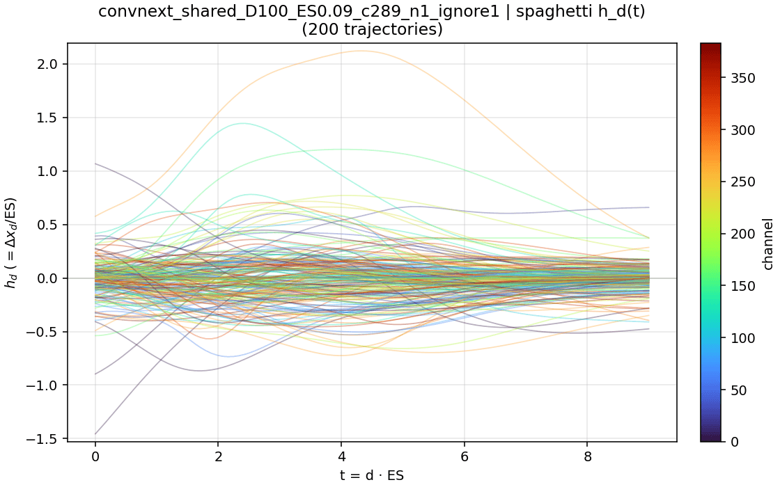
You can see it in the residual field. Each curve below is one channel of h = Δx/Δt, averaged over space, along the nine blocks of ConvNeXt-T at R = 100, for a single validation image (a snow leopard).
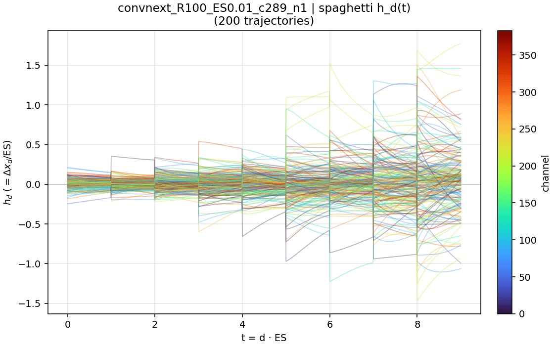
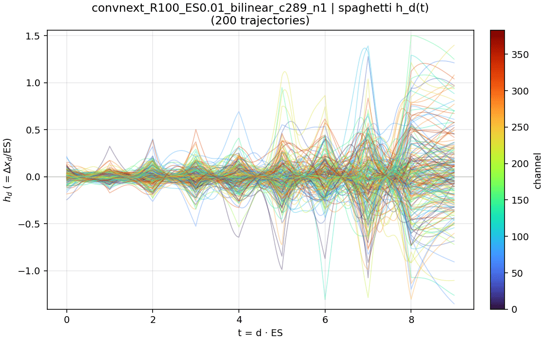
In numbers, measured over 500 images: bilinear keeps the global shape of the trajectory (its straightness and dimensionality barely change) but multiplies local curvature by 6 to 12 and angular speed by 4 to 7, and doubles the distance to the native trajectory.
4. One block for the whole stage
If stage 3 really integrates a smooth flow, one block should be able to define the vector field for the whole stage. So I trained a ConvNeXt-T in which the nine stage-3 blocks are the same block applied nine times, with the same recipe as the baseline: 300 epochs on ImageNet-1k. Weight sharing across depth is not new [17, 18], but here it is a direct test of the ODE reading.
- ConvNeXt-T
- ConvNeXt-T, no drop path
- Shared stage 3 (1 block × 9)
The shared network reaches 80.34% against 80.96%, a cost of 0.62 points. Stage 3 goes from nine blocks to one, which removes about 9.6M of ConvNeXt-T's 28.6M parameters.
Accuracy depends on the integration time, not on the number of steps
With a single field, depth D and step Δt can be chosen freely at inference, and the integration time is T = D · Δt. The network was trained with D = 9 and Δt = 1, so T = 9. Keeping T = 9 and changing D:
- Euler (RK1)
- RK2
- RK4
The gap from Euler to the continuous limit is −0.22 points, three times smaller than in the unshared ConvNeXt (−0.73): sharing weights produces a more genuine ODE. With large steps the order of the solver matters a lot. At D = 4, RK4 gets 78.9% and Euler 67.8%, and Euler with two steps of 4.5 is unstable (5.9%). RK4 reaches the limit from D ≈ 5, RK2 from about 18 and Euler only from about 256.
- Fixed step 1, more steps (T = D)
- 9 steps, varying step size (T = 9 · step)
Integrating too short or too long degrades smoothly near T = 9 and collapses far from it: 49% at T = 32 with unit steps, and 0.3% at T = 128. The classification head expects the state reached after exactly that much time.
5. Why expand: depth at higher resolution
The original ConvNeXt-T shows you stage 3 in ten frames: the input and the output of each of the nine blocks. Everything that happens inside a block is invisible. That is a problem, because the questions worth asking about dynamics are questions about derivatives. How fast does the representation move? Does it accelerate or brake? Does it go straight or turn? When is each feature decided? With ten samples of a path in 75,264 dimensions (384 channels × 14 × 14), a finite difference across a block mixes two different things: the motion inside the block, and the change of vector field when the next block takes over. A second difference, which is what acceleration and curvature need, is hopeless.
Expanding the skip connections is the equivalent of switching to a high-speed camera. With , the same stage is sampled at 901 states, every . Two things make those extra frames trustworthy rather than made up. The function is preserved: accuracy stays within 0.6 to 0.9 points of the original (section 2). And the refined path stays close to the original states, measured on 500 images:
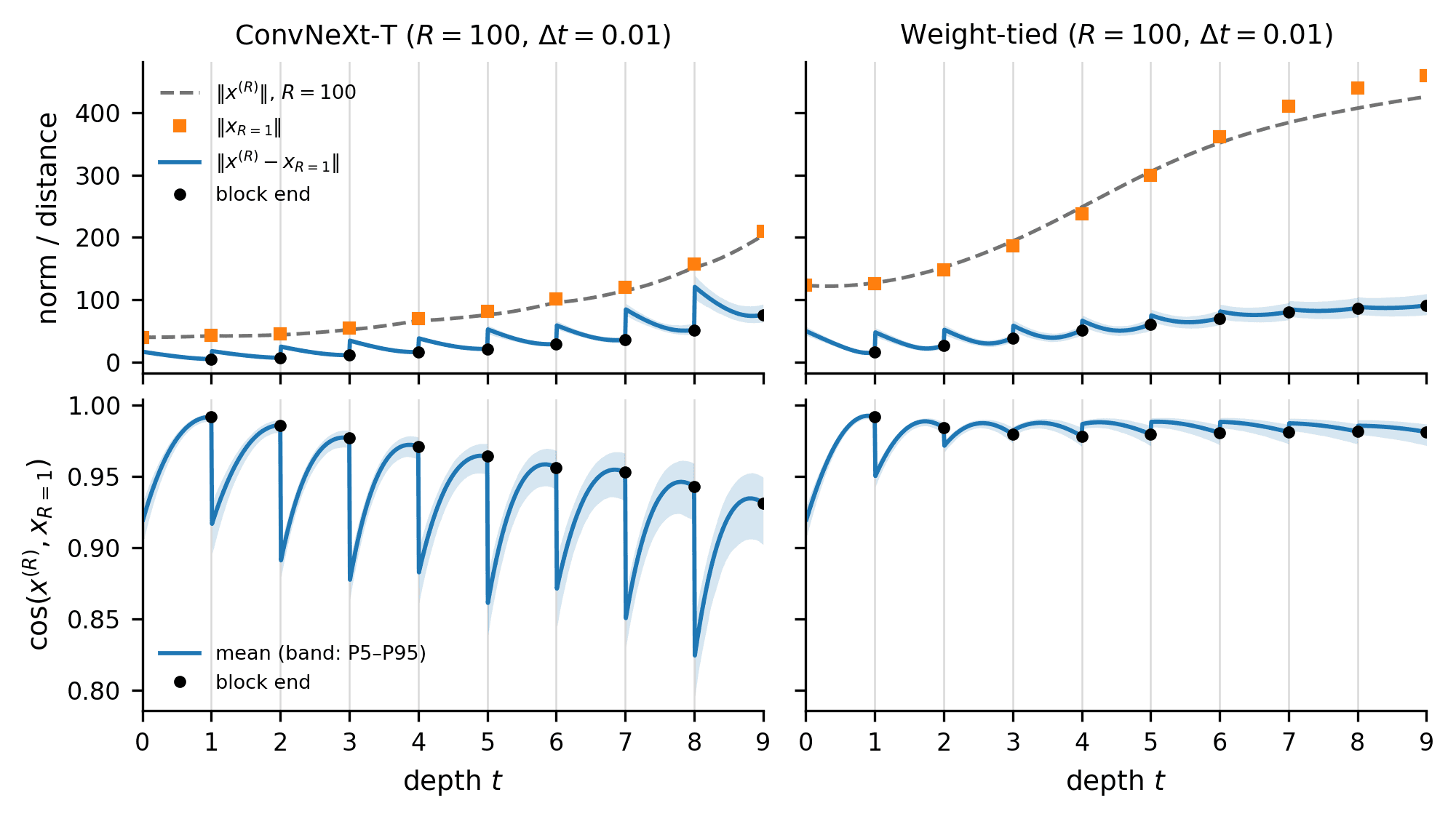
The speed of the point
The simplest thing to measure is how fast the point moves: the length of the arrow under it, . It is the velocity field read along the trajectory, not the field itself, which lives in all 75,264 dimensions and has an arrow at every location. Here it is over 500 images, with every channel included.
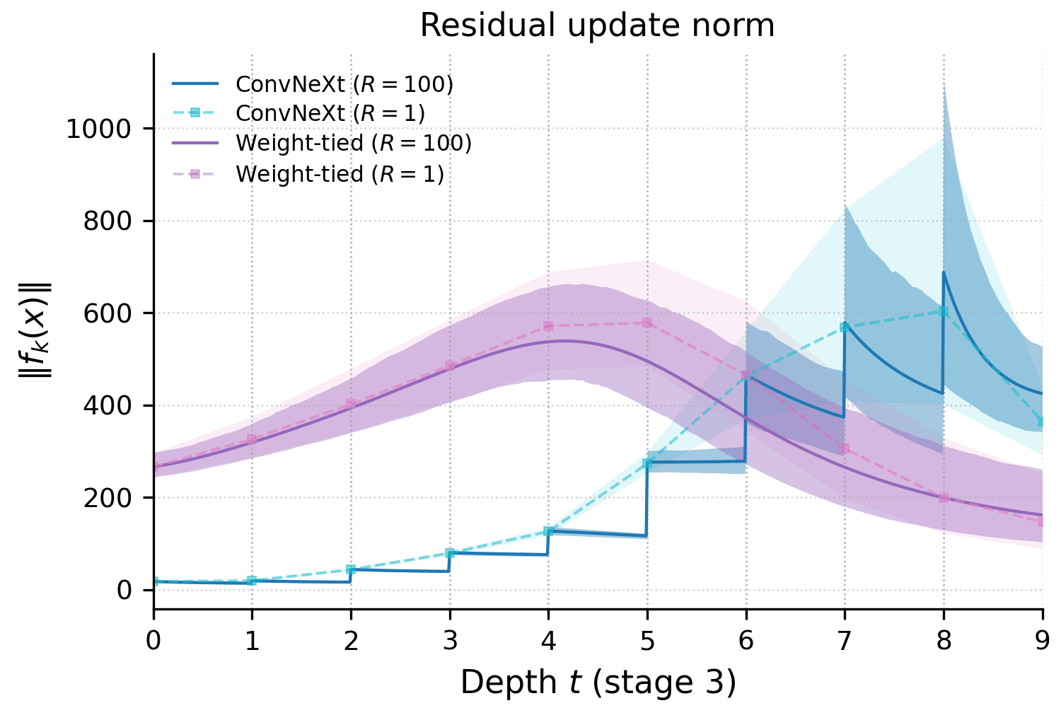
In the weight-tied network the speed is one bell: about 270 at the entrance of the stage, a peak of about 540 around , and down to 160 at the exit. The curve is continuous because the field is autonomous. The arrows never change; the point only speeds up or slows down because it moves into regions where the arrows are longer or shorter. The one-step-per-block markers sit on that curve, overshooting slightly at the peak (about 570 against 540), which is the error of a coarse Euler step.
The original network is where the expansion earns its keep. With one step per block (dashed), its speed looks like a smooth growth from 18 to 600 over eight blocks, a point that keeps accelerating. With 100 steps per block (solid) that picture turns out to be false. The speed is a sawtooth: it jumps up at every block switch, and inside the block it never grows. In the first blocks it stays flat; in the last ones it decays. In the final block it falls from 690 to 425, so the point leaves the stage almost 40% slower than it entered that block. Inside a block the point brakes or coasts; what accelerates it is the switch to a new field. The dashed curve, which is all the original network lets you see, hides the braking completely. The band also widens in the last three blocks: how fast the point moves at the end depends on the image much more than at the beginning, consistent with a network that commits late.
These numbers are dominated by the massive channel of section 7, which is why they are about ten times larger than the speeds in Figure 1, and why the shared network already starts at 270. Without the channel the shapes survive: a bell from 50 to 75 and back to 42 in the shared network, and steps from 17 to more than 100 in the original one (Figure 1, bottom).
Coordinate by coordinate
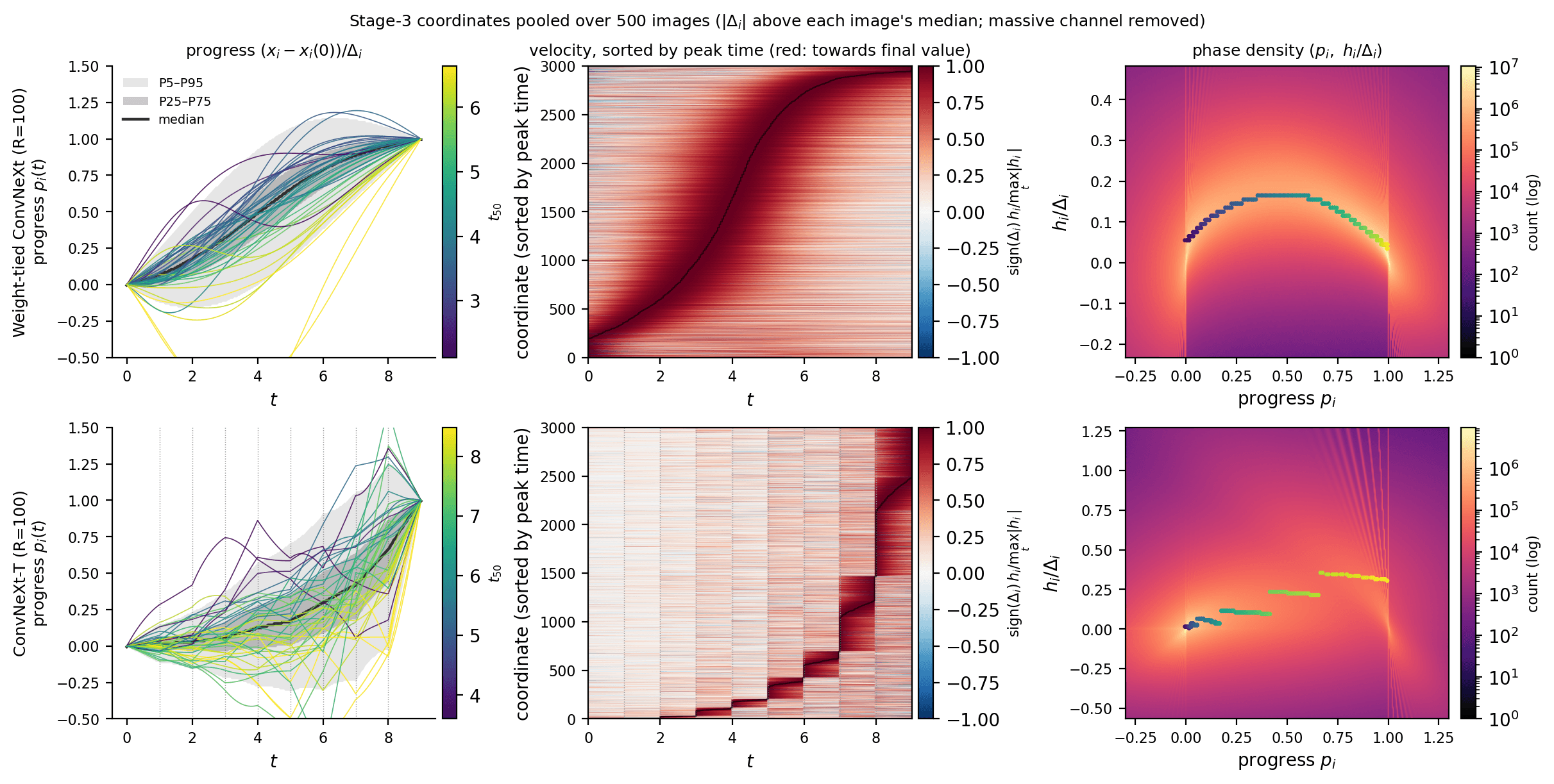
The extra resolution is not a cosmetic upgrade. It decides what you conclude. The figure below follows individual coordinates of the stage-3 state, pooled over the same 500 images. For each image I keep the coordinates whose total change is above that image's median, and normalise each one to its own journey:
is the progress of coordinate : 0 where it starts, 1 at its final value. is its velocity in the same units, positive when it moves towards its final value. is the first time a coordinate is half-way there.
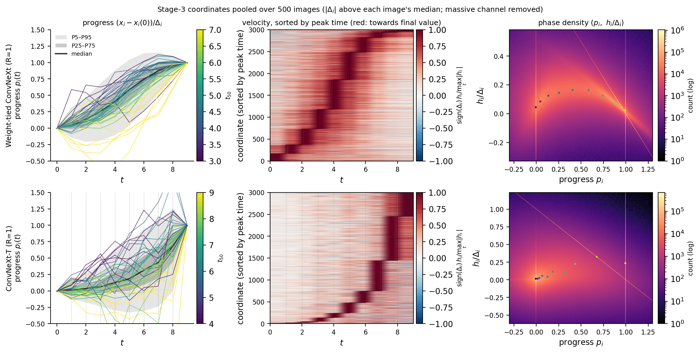
At one step per block, both networks look like staircases. In the raster, every coordinate seems to be switched on by one particular block, and the phase plane is nine scattered dots. From those pictures alone you could not tell a smooth flow sampled coarsely from a sequence of unrelated maps.
At the two networks separate. The shared network becomes a single continuous wave: coordinates are recruited at staggered times (median = 4.1), each one launches, peaks and brakes as it approaches its final value, and the whole population traces one arch in the phase plane. The stage is a flow with a beginning, a middle and an end, and the staircase was an artefact of sampling it every unit of time. The original ConvNeXt-T keeps its steps, now resolved: inside a block the velocity of each coordinate barely changes direction, and every discontinuity sits exactly at a block boundary. In the phase plane each block draws its own short arc, starting where the previous one stopped but at a different velocity. Across a boundary, 44.6% of the coordinates flip the sign of their velocity. Inside a block, from one step of 0.01 to the next, it is about 0.2%. In the shared network the flip rate at integer times is 0.1%, because nothing special happens there.
That is the use of interpolating depth: it separates what the network does from how coarsely we were looking at it. The jumps of the original network are real, the steps of the shared network are not, and only the refined trajectories can tell them apart.
6. What the trajectories look like
To compare networks beyond accuracy I measure the geometry of the path the state takes through stage 3: norms of and , angular speed of , tangential and normal acceleration, curvature, straightness (net displacement over path length; 1 for a straight line), and the participation ratio of the trajectory, its effective number of dimensions. Everything was first computed on one image (ImageNet val #644, a snow leopard), then repeated on a suite of 500 validation images, one from each of 500 random classes (seed 0; the same 500 images in every run).
The single image was representative. Every metric of that image falls within about 1.5 standard deviations of the 500-image mean, and the spread between images is small (). The geometry belongs to the network, not to the input. The numbers in the tables below are that N=500 mean.
Two ways of moving through a stage
Figure 1 coloured the trajectories by time. Coloured by class, they show where each image is going. In the shared network every class leaves a common origin and fans out along its own smooth curve, and the final states alone already separate the classes. In the original network the classes separate too, but the paths bend at every block boundary.
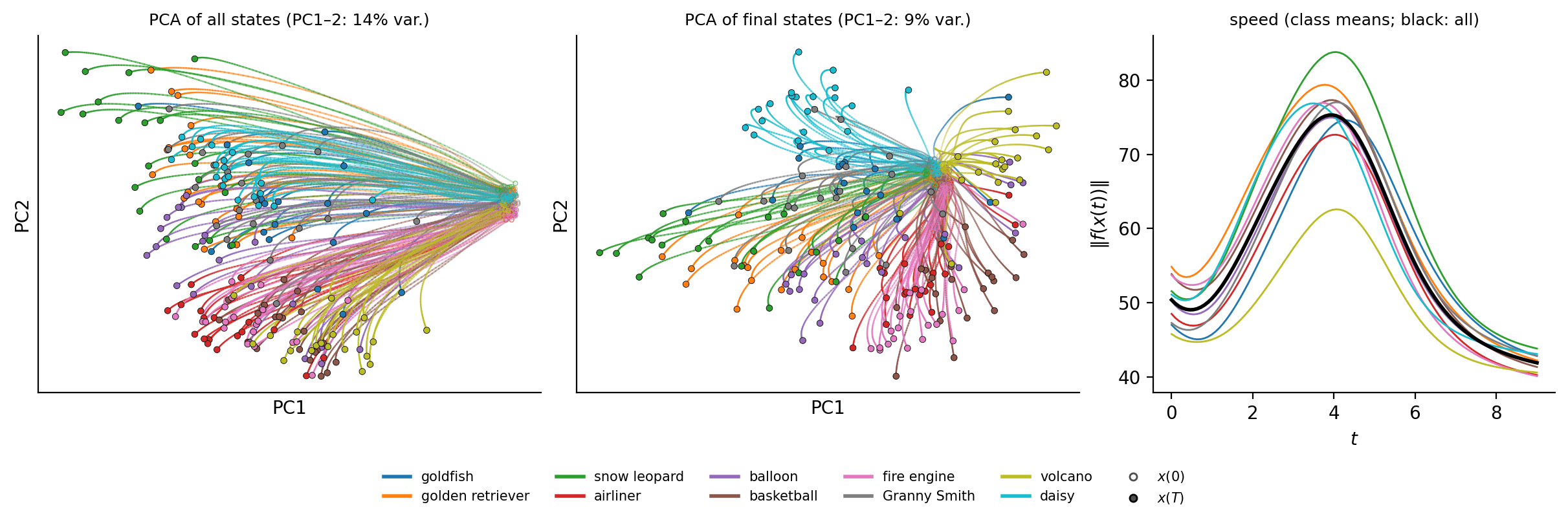
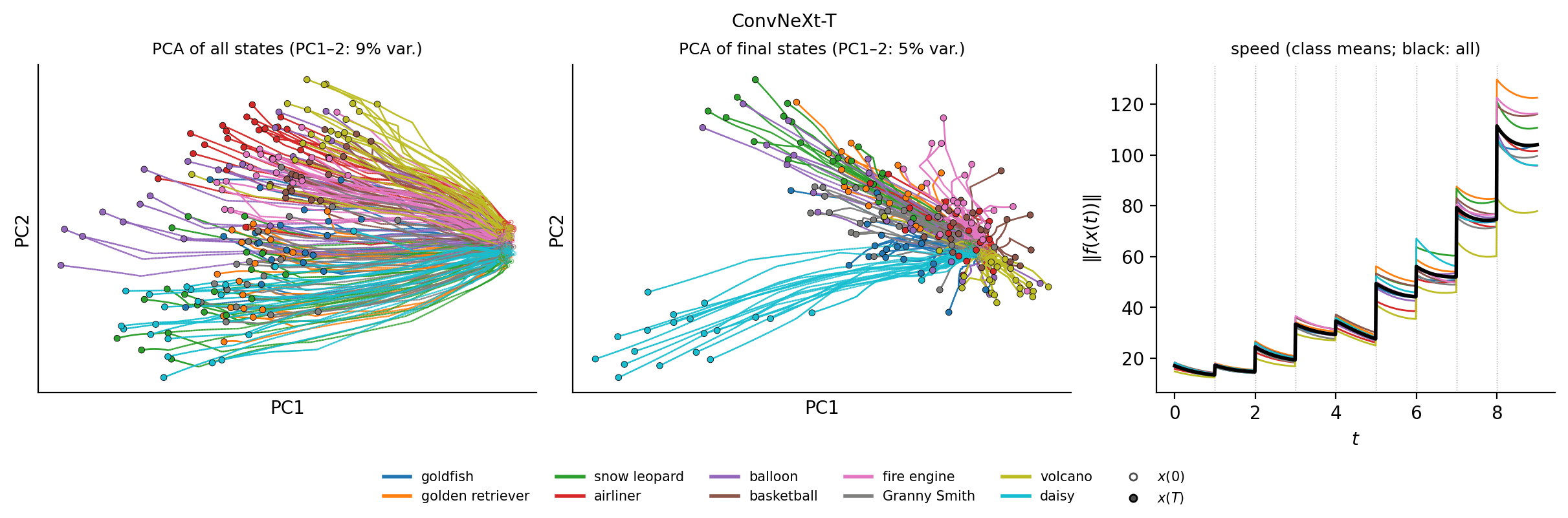
The videos make the contrast concrete. On the left of each, the shared network; on the right, the original one, integrated over the same nine units of depth and played in sync.
Independent blocks undo each other
Look again at the ConvNeXt-T rows of Figure 11. The median coordinate of the original network does not progress smoothly: many coordinates overshoot, come back, and go out again, and most of them only commit to their final value in the last two blocks (median = 7.2). To quantify it, take the displacement of each block, , coordinate by coordinate:
| Model | R | Straightness | Wasted motion | Monotone share | cos(Δxₖ, Δxₖ₊₁) | Reversal rate | Undo fraction | Zig-zag share | Median t₅₀ | Top-1 (500 img.) |
|---|---|---|---|---|---|---|---|---|---|---|
| Shared stage 3 | 100 | 0.78 | 19% | 73% | 0.92 | 11% | 2% | 14% | 4.1 | 80.8% |
| Shared stage 3 | 1 | 0.72 | 25% | 63% | 0.77 | 18% | 5% | 34% | 5.0 | 81.2% |
| ConvNeXt-T | 100 | 0.50 | 48% | 21% | 0.17 | 45% | 25% | 90% | 7.2 | 81.2% |
| ConvNeXt-T | 1 | 0.50 | 48% | 22% | 0.17 | 45% | 25% | 90% | 7.8 | 80.0% |
N=500, massive channel removed. Wasted motion: 1 − |net displacement| / Σ|block displacements|, summed over coordinates. Monotone share: fraction of the total change carried by coordinates that move backwards less than 5% of their path. Reversal rate: fraction of coordinates whose displacement changes sign from one block to the next (50% would be a coin flip). Undo fraction: share of a block's displacement cancelled by the next block. Zig-zag share: fraction of block displacement in coordinates that reverse at least twice.
Consecutive blocks of the original ConvNeXt-T push the state in nearly orthogonal directions (cosine 0.17; two random directions in this space would give about 0.004, so they are related, but barely). From one block to the next, 45% of the coordinates reverse, close to the 50% of a coin flip, and a quarter of what each block moves is cancelled by the following one. 90% of the block-level motion is in coordinates that zig-zag at least twice, and in total half of the distance travelled coordinate by coordinate cancels out. The shared network, at the same accuracy, wastes 19%, and 73% of its change is carried by coordinates that move monotonically to their final value.
These numbers are the same at and for the original network, so the zig-zag is a property of the trained blocks, not of the refinement. The shared network at looks somewhat worse than at , which is the coarse Euler step overshooting a flow that is really smooth.
On average, all blocks do push towards the final representation; the median curve rises. Coordinate by coordinate, they do not. Nine independent blocks reach the same accuracy as one shared field by building and destroying a large part of what the previous block wrote. Why they do this is open. They may use some coordinates as temporary workspace, or overparametrisation may simply let each block correct its predecessor. What the shared network shows is that the zig-zag is not needed to classify well.
One image, all channels

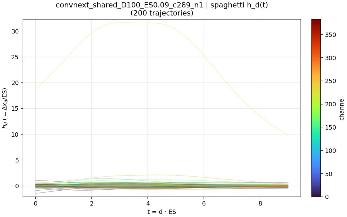
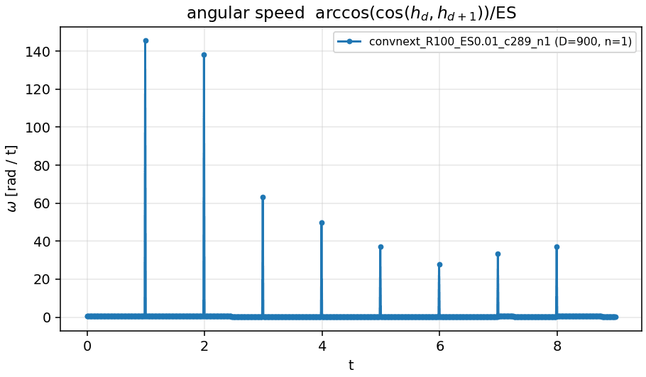
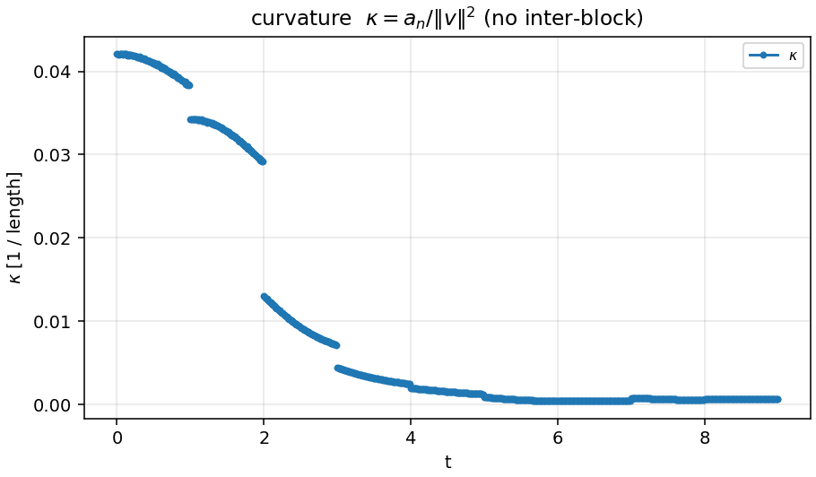
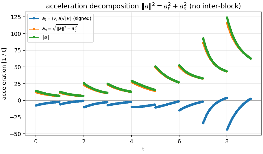
With all channels included, every ConvNeXt looks like an almost perfectly straight, one-dimensional flow, and there is a clear ranking: shared, then ConvNeXt, then Swin, then the ResNets. ResNet-101 follows a very tortuous path in about 20 effective dimensions. The unshared ConvNeXt shows a sawtooth pattern: inside each block h contracts, and at each block boundary it jumps by 10² to 10⁴ times the within-block acceleration.
Dynamics and geometry
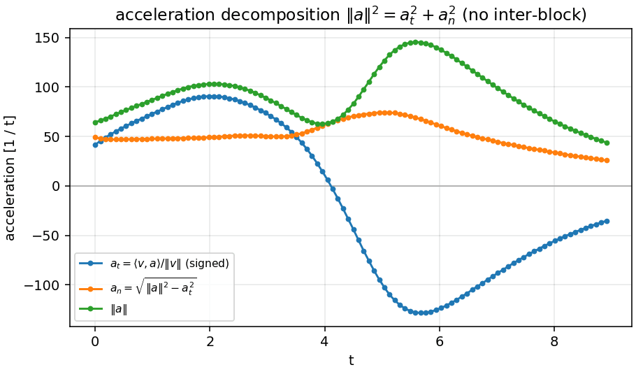
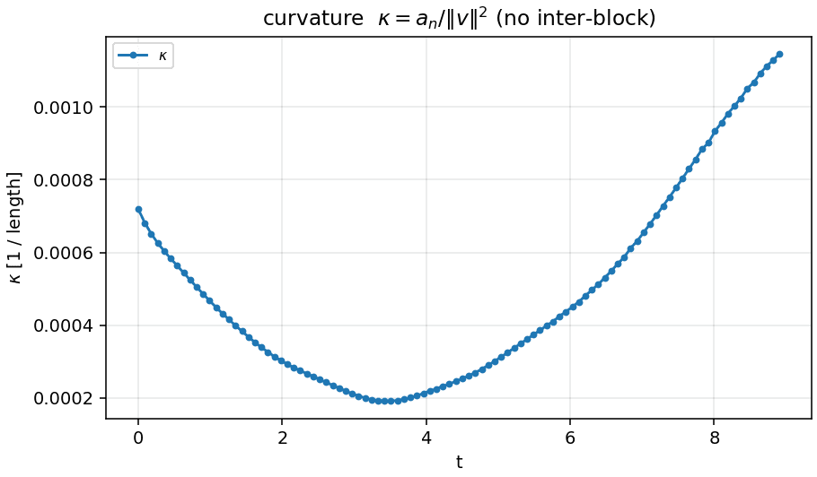
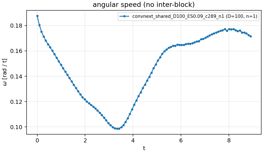
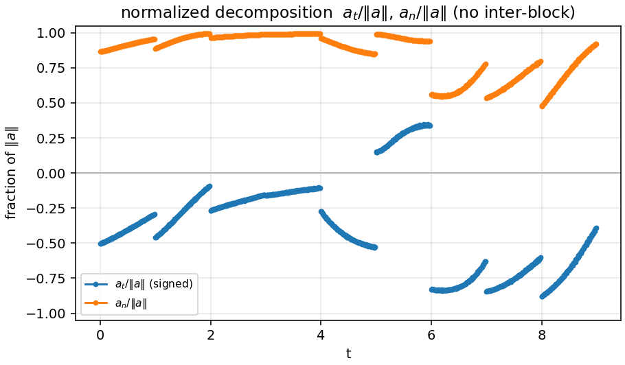
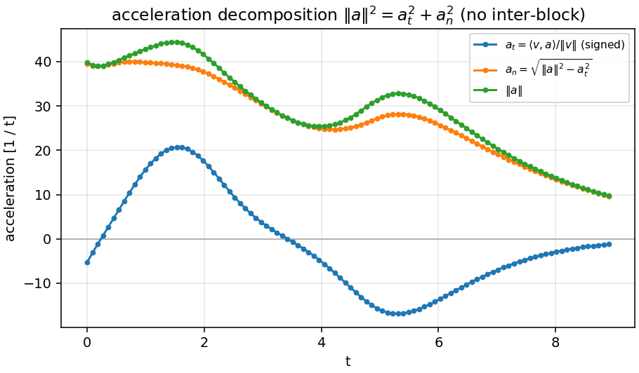
Write for the residual velocity and for its acceleration. The tangential and normal parts are
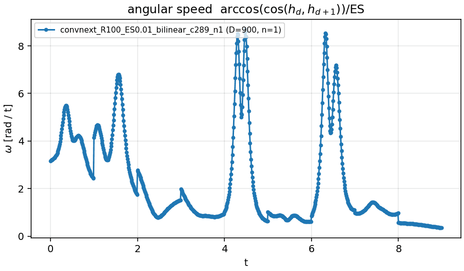
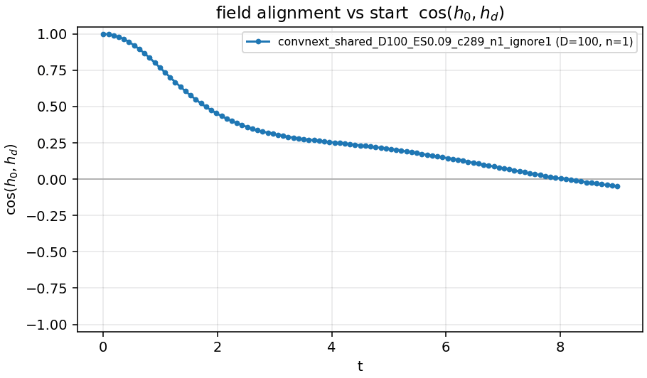
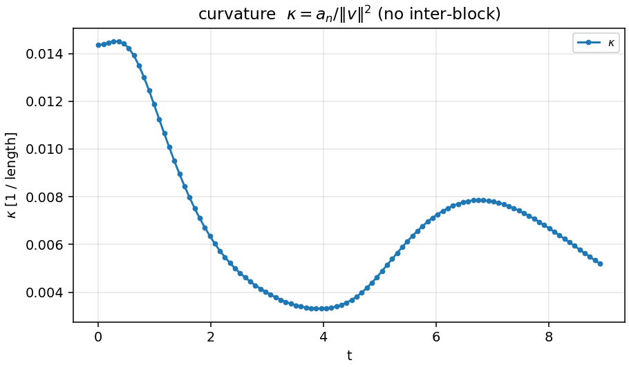
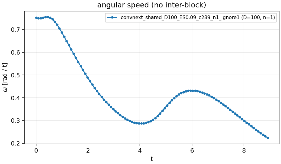
is signed: negative means the trajectory is braking ( shrinks). is a norm, so always positive, and . Angular speed is . The panels below drop the single step between blocks, so they show the intra-block flow; the panel that keeps those steps is labelled as such.
7. Massive activations and the ignore path
The straight lines are mostly one channel: a massive activation [19]. At the exit of stage 3 in the shared network, channel 236 has a norm of 3,570; the next largest has 140. It is the same channel in all 200 images I checked, and it holds a median 98% of the energy of the state.
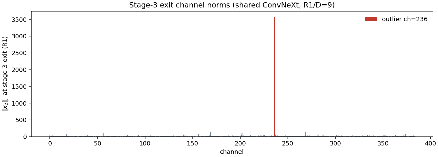
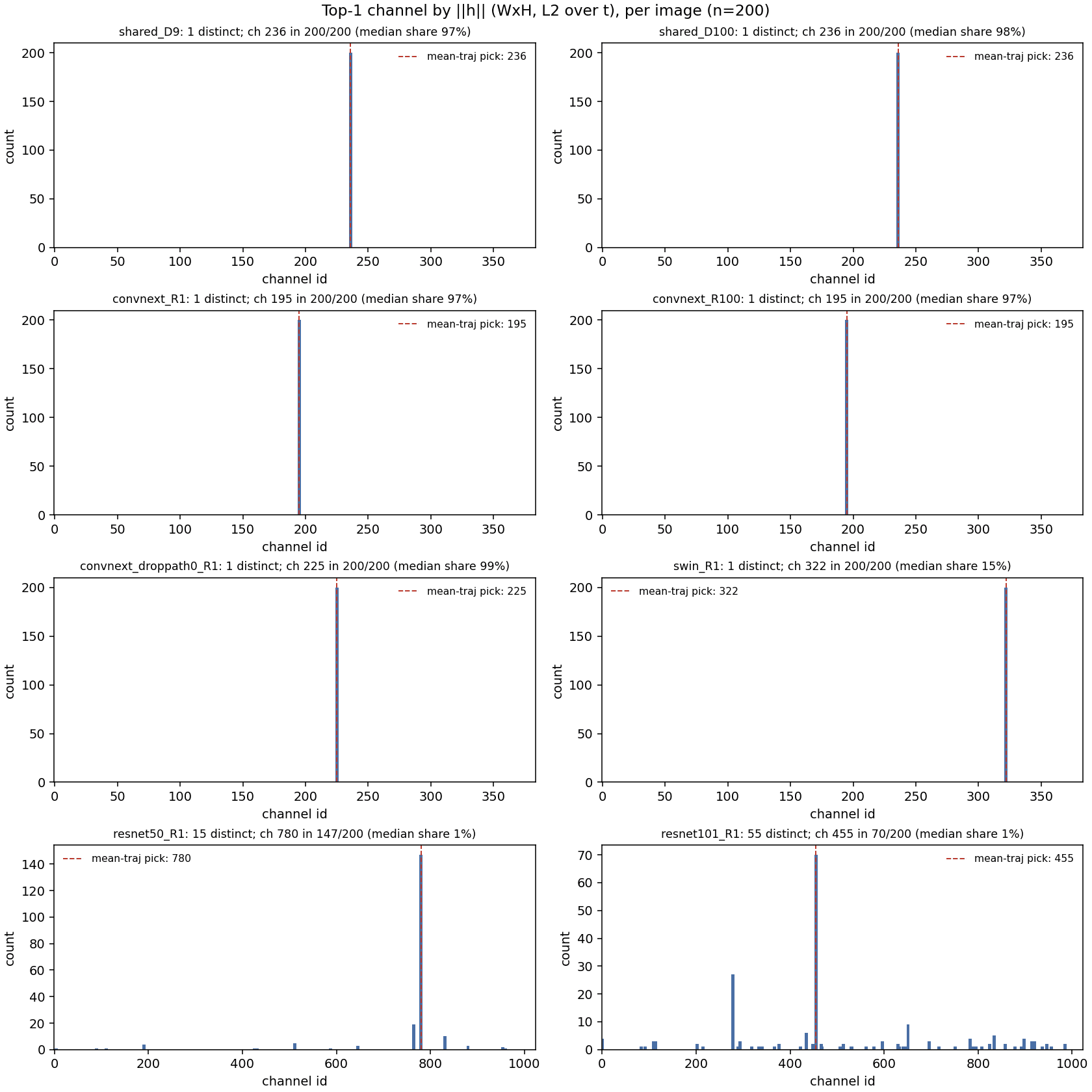
The same phenomenon appears in all three ConvNeXts (channels 236, 195 and 225, with 97 to 99% of the energy). Swin has a moderate one, at about 15%, and the ResNets have none: their top channel changes from image to image and carries about 1%. They are close relatives of the high-norm tokens in vision transformers [20]. One difference: in the shared network the channel dominates from the first step, while in the unshared ConvNeXt it emerges with depth, from 5% of at the start to 96% at the end.
The ignore path: drop the channel from the metric, not from the ODE
The ignore path (_ignore1 in the experiment suite) leaves the network untouched and only removes the massive channel when the trajectory metrics are computed. That is not the same as zeroing the channel inside the residual step, which I come back to below. On N=500, ignoring it changes ConvNeXt completely and Swin almost not at all.
| Model | Ignore | R | σ(R) | PR depth | PR spatial | κ | ω | aₙ/‖a‖ | aₜ/‖a‖ | cos(x₀,x_T) | cos(h₀,h_T) |
|---|---|---|---|---|---|---|---|---|---|---|---|
| Shared stage 3 | — | 0.970 | 0.008 | 1.09 | 1.03 | 0.0005 | 0.15 | 0.58 | -0.07 | 0.67 | 0.73 |
| Shared stage 3 | ch 236 | 0.776 | 0.020 | 1.94 | 6.24 | 0.0075 | 0.41 | 0.95 | -0.06 | 0.31 | -0.06 |
| ConvNeXt-T | — | 0.938 | 0.010 | 1.19 | 1.13 | 0.0098 | 0.34 | 0.87 | -0.38 | 0.48 | 0.17 |
| ConvNeXt-T | ch 195 | 0.502 | 0.011 | 3.46 | 32.00 | 0.0210 | 0.61 | 0.97 | -0.21 | 0.21 | 0.02 |
| ConvNeXt-T, no drop path | — | 0.934 | 0.010 | 1.04 | 8.76 | 0.0200 | 0.56 | 0.96 | 0.04 | 0.33 | 0.27 |
| ConvNeXt-T, no drop path | ch 225 | 0.438 | 0.012 | 3.20 | 29.50 | 0.0280 | 0.84 | 0.98 | 0.10 | 0.17 | 0.01 |
| Swin-T | — | 0.825 | 0.014 | 1.17 | 6.15 | 0.0042 | 0.50 | 0.89 | -0.39 | 0.09 | 0.04 |
| Swin-T | ch 322 | 0.812 | 0.016 | 1.17 | 7.31 | 0.0044 | 0.51 | 0.89 | -0.39 | 0.08 | 0.03 |
| ResNet-50 | — | 0.396 | 0.012 | 4.94 | 5.84 | 0.0024 | 0.63 | 0.90 | -0.41 | 0.60 | -0.08 |
| ResNet-101 | — | 0.169 | 0.005 | 19.66 | 12.10 | 0.0022 | 0.54 | 0.93 | -0.31 | 0.48 | -0.04 |
N=500, one ImageNet validation image per class, same 500 images in every run. Fine Euler (R=100 or D=100). R is straightness (N/L). κ and ω are intra-block means. ResNets have no massive channel, so there is no ignore path for them.
With every channel, the ranking in straightness is shared 0.97 > ConvNeXt 0.94 ≈ no-drop-path 0.93 > Swin 0.83 > ResNet-50 0.40 > ResNet-101 0.17. After the ignore path it becomes Swin 0.81 > shared 0.78 > ConvNeXt 0.50 > no-drop-path 0.44 > ResNet-50 0.40 > ResNet-101 0.17. The unshared ConvNeXt without its channel is almost as tortuous as ResNet-50; Swin is the unshared network whose straightness is real. In the shared network more than 90% of the acceleration becomes normal: rotates until it ends up orthogonal to where it started (), while fades from 0.42 to 0.09. A drift that turns and dies out.
Zeroing versus ignoring
Zeroing writes the channel to 0 after every residual step of the shared network, so the ODE itself changes. That drops accuracy from 80.34% to 67.81%. Zeroing a random channel instead costs nothing (mean 80.25% over 20 channels). The same holds at ten times the resolution (from 80.14% to 67.59%).
The ignore path and this zeroing agree on the other 383 channels to within 0.5% on every metric (straightness 0.7944 vs 0.7947, path length, participation ratios, mean curvature). The channel does not feed back into the rest of the stage-3 field, so it is not an internal clock that reads. Its effect is downstream: holding 98% of the energy, it sets the variance that the LayerNorm before downsampling divides by. Remove it and the scale of everything else changes about 7×, a distribution shift for stage 4. Whether it carries information about the image, or acts as a near-constant bias and scale, is still open.
8. Shared block plus per-block deltas
Section 6 suggests that nine independent blocks are a wasteful way to integrate a stage: they carry a common flow plus large, mutually cancelling corrections. Sharing removes the waste but costs 0.6 points. The natural question is whether a shared flow with small per-block corrections can close that gap. Each block k gets its own offset on top of the shared weights:
The deltas cover every parameter of the block: depthwise convolution, LayerNorm, both pointwise layers and the layer scale. They start at zero from the shared checkpoint, so epoch 0 is exactly the shared network, and they have their own weight decay pulling them back towards it. Then the whole model is fine-tuned.
- Δ, 9 steps, peak LR 1e-3, 50 epochs
- Δ, 9 steps, peak LR 1e-4, 100 epochs
- Δ, unrolled to 27 steps of 1/3, LR 1e-5 (running)
With a peak learning rate of 10⁻³ for 50 epochs, the delta model reaches 81.25%, +0.91 over the shared network and +0.29 over the original. A gentler schedule (10⁻⁴, 100 epochs) stays at 80.57%. The deltas do not stay small. By the end of the best run they average 27% of the norm of the shared weights.
- mean ‖δₖ‖ / ‖θ_shared‖ over blocks and layers
Two caveats, to be fair to the baseline. The delta model has as many stage-3 parameters as the original plus one block, so it is a reparametrisation, not a compression. And it has seen 50 more epochs than the original. What it shows is that a shared field plus per-block corrections is a better starting point than nine independent blocks. Whether the deltas can be made sparse or low-rank, recovering the parameter savings, is the next step.
9. Is drop path the reason?
Stochastic depth [21] randomly skips blocks during training, so every block has to be optional. That should push towards small updates that agree with their neighbours, which is what an ODE needs. Residual networks are already known to tolerate dropped and reordered layers [22, 23, 24]. ConvNeXt-T trained without drop path tests the idea directly:
| With drop path 0.1 | Without | Difference | |
|---|---|---|---|
| Original accuracy | 80.96 | 79.27 | −1.69 |
| ODE limit (RK4) | 80.23 | 76.96 | −3.27 |
| Gap to the limit | −0.73 | −2.31 | 3.2× larger |
| Bilinear, R = 128 | 73.66 | 57.44 | −16.2 |
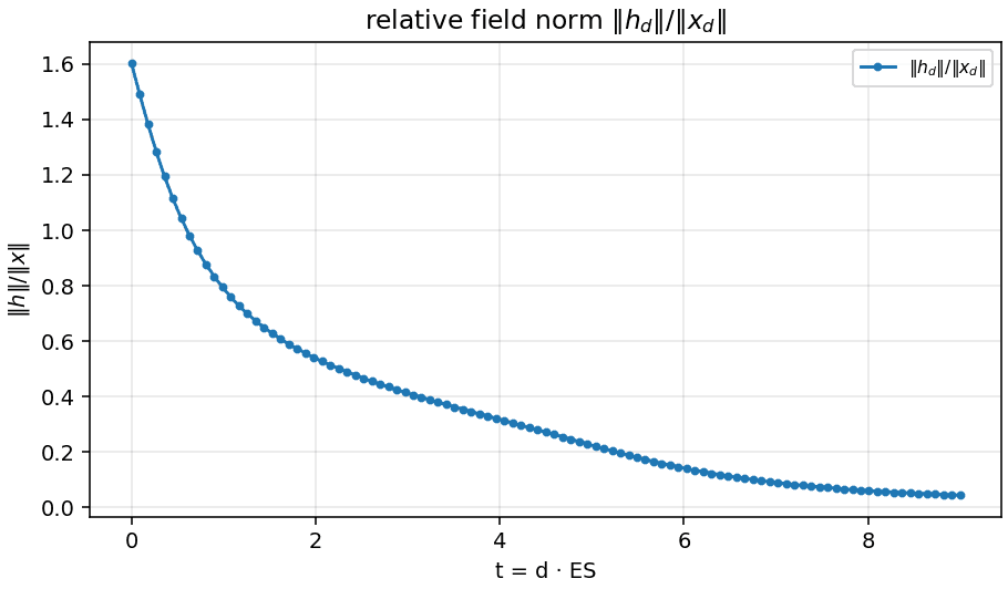
Without drop path, the gap to the continuous limit triples, bilinear interpolation collapses, and the blocks stop contracting. It is the only network whose trajectory accelerates inside each block and whose ‖h‖/‖x‖ grows with depth, from 0.39 to 0.65. But drop path is not a necessary condition, since Swin and both ResNets converge with similar gaps. The Euler-like behaviour seems to be generic to deep residual networks, and drop path strengthens it.
10. Open questions
- Finish the 27-step delta run, and the shared networks with 27 steps and with every stage shared, and run the depth, step and solver ablations on them.
- Make the deltas sparse or low-rank, so the delta model recovers the parameter savings of sharing.
- Explain the zig-zag of independent blocks: which coordinates are built and destroyed, whether they carry information that a later block reads, and whether the delta model inherits it or stays close to the shared flow.
- Pin down the massive channel. Replace it by its dataset mean instead of zero, which separates bias from information. Replace it by its value at a different time, which tests a clock read by stage 4. Zero it only at the exit of stage 3. Fit a linear probe of the class on it.
- Repeat the zeroing on the unshared ConvNeXt and on Swin, where the channel emerges with depth.
- Close the causal question about drop path with intermediate rates and a shared network trained without it.
- Interpolate in function space, (1 − α) fk(x) + α fk+1(x), which needs no weight alignment, or in weight space after aligning consecutive blocks [16].
The training framework and the from-scratch ConvNeXt run this builds on are written up in ConvNeXt-V1 from scratch on Leonardo. If you work on continuous-depth models or massive activations and want to compare notes, write to jaume@jaumeivars.com.
References
- [1]K. He, X. Zhang, S. Ren, J. Sun. Deep Residual Learning for Image Recognition. CVPR, 2016.
- [2]W. E. A Proposal on Machine Learning via Dynamical Systems. Communications in Mathematics and Statistics 5(1), 2017.
- [3]E. Haber, L. Ruthotto. Stable Architectures for Deep Neural Networks. Inverse Problems 34(1), 2017.
- [4]Y. Lu, A. Zhong, Q. Li, B. Dong. Beyond Finite Layer Neural Networks: Bridging Deep Architectures and Numerical Differential Equations. ICML, 2018.
- [5]R. T. Q. Chen, Y. Rubanova, J. Bettencourt, D. Duvenaud. Neural Ordinary Differential Equations. NeurIPS, 2018.
- [6]M. E. Sander, P. Ablin, G. Peyré. Do Residual Neural Networks discretize Neural Ordinary Differential Equations? NeurIPS, 2022.
- [7]Z. Liu, H. Mao, C.-Y. Wu, C. Feichtenhofer, T. Darrell, S. Xie. A ConvNet for the 2020s. CVPR, 2022.
- [8]Z. Liu, Y. Lin, Y. Cao, H. Hu, Y. Wei, Z. Zhang, S. Lin, B. Guo. Swin Transformer: Hierarchical Vision Transformer using Shifted Windows. ICCV, 2021.
- [9]E. Hairer, S. P. Nørsett, G. Wanner. Solving Ordinary Differential Equations I: Nonstiff Problems (2nd ed.). Springer, 1993.
- [10]B. Chang, L. Meng, E. Haber, F. Tung, D. Begert. Multi-level Residual Networks from Dynamical Systems View. ICLR, 2018.
- [11]A. F. Queiruga, N. B. Erichson, D. Taylor, M. W. Mahoney. Continuous-in-Depth Neural Networks. arXiv preprint, 2020.
- [12]J. Deng, W. Dong, R. Socher, L.-J. Li, K. Li, L. Fei-Fei. ImageNet: A Large-Scale Hierarchical Image Database. CVPR, 2009.
- [13]R. Wightman. PyTorch Image Models. GitHub repository, 2019.
- [14]TorchVision maintainers and contributors. TorchVision: PyTorch's Computer Vision library. GitHub repository, 2016.
- [15]R. Entezari, H. Sedghi, O. Saukh, B. Neyshabur. The Role of Permutation Invariance in Linear Mode Connectivity of Neural Networks. ICLR, 2022.
- [16]S. K. Ainsworth, J. Hayase, S. Srinivasa. Git Re-Basin: Merging Models modulo Permutation Symmetries. ICLR, 2023.
- [17]M. Dehghani, S. Gouws, O. Vinyals, J. Uszkoreit, Ł. Kaiser. Universal Transformers. ICLR, 2019.
- [18]Z. Lan, M. Chen, S. Goodman, K. Gimpel, P. Sharma, R. Soricut. ALBERT: A Lite BERT for Self-supervised Learning of Language Representations. ICLR, 2020.
- [19]M. Sun, X. Chen, J. Z. Kolter, Z. Liu. Massive Activations in Large Language Models. COLM, 2024.
- [20]T. Darcet, M. Oquab, J. Mairal, P. Bojanowski. Vision Transformers Need Registers. ICLR, 2024.
- [21]G. Huang, Y. Sun, Z. Liu, D. Sedra, K. Q. Weinberger. Deep Networks with Stochastic Depth. ECCV, 2016.
- [22]A. Veit, M. Wilber, S. Belongie. Residual Networks Behave Like Ensembles of Relatively Shallow Networks. NeurIPS, 2016.
- [23]K. Greff, R. K. Srivastava, J. Schmidhuber. Highway and Residual Networks learn Unrolled Iterative Estimation. ICLR, 2017.
- [24]S. Jastrzębski, D. Arpit, N. Ballas, V. Verma, T. Che, Y. Bengio. Residual Connections Encourage Iterative Inference. ICLR, 2018.